H2020-MSCA-IF-2019, Example: ground states
This page details how to obtain homogeneous solutions of BFO for the structural and spin order. The first calculation (BFO_homogeneous_PA.i) determines the polarization and antiphase octahedral cage tilt vectors along with the coupled elastic strain tensor components computed from the elastic displacement variable .
The second (BFO_P0A0_mRD.i) uses information from the first to determine the antiferromagnetic order corresponding to the Neel vector and total magnetization . We can separate these calculations because the magnetic system does not appreciably influence the relaxation dynamics of the polarization since the work required to move ions (i.e. those relative displacements corresponding to and ) is much larger than those to reorient the Fe spins.
Homogeneous structural order
We first consider a simple nm on a grid of finite elements with the Mesh block,
[Mesh]
  [gen]
    type = GeneratedMeshGenerator
    dim = 3
    nx = ${Nx}
    ny = ${Ny}
    nz = ${Nz}
    xmin = 0.0
    xmax = ${xMax}
    ymin = 0.0
    ymax = ${yMax}
    zmin = 0.0
    zmax = ${zMax}
    elem_type = HEX8
  []
  [./cnode]
    input = gen

    ############################################
    ##
    ##   additional boundary sideset (one node)
    ##   to zero one of the elastic displacement vectors
    ##   vectors and eliminates rigid body translations
    ##   from the degrees of freedom
    ##
    ##   NOTE: This must conform with the about
    ##         [Mesh] block settings
    ##
    ############################################

    type = ExtraNodesetGenerator
    coord = '0.0 0.0 0.0'
    new_boundary = 100
  [../]
[]
The Variables block defines the relevant variables of the simulation,
[Variables]
  [./u_x]
  [../]
  [./u_y]
  [../]
  [./u_z]
  [../]
  [./global_strain]
    order = SIXTH
    family = SCALAR
  [../]
  [./polar_x]
    order = FIRST
    family = LAGRANGE
    [./InitialCondition]
      type = FunctionIC
      function = constPp
    [../]
  [../]
  [./polar_y]
    order = FIRST
    family = LAGRANGE
    [./InitialCondition]
      type = FunctionIC
      function = constPp
    [../]
  [../]
  [./polar_z]
    order = FIRST
    family = LAGRANGE
    [./InitialCondition]
      type = FunctionIC
      function = constPm
    [../]
  [../]
  [./antiphase_A_x]
    order = FIRST
    family = LAGRANGE
    [./InitialCondition]
      type = FunctionIC
      function = constAp
    [../]
  [../]
  [./antiphase_A_y]
    order = FIRST
    family = LAGRANGE
    [./InitialCondition]
      type = FunctionIC
      function = constAp
    [../]
  [../]
  [./antiphase_A_z]
    order = FIRST
    family = LAGRANGE
    [./InitialCondition]
      type = FunctionIC
      function = constAm
    [../]
  [../]

  [./potential_E_int]
    order = FIRST
    family = LAGRANGE
  [../]
[]
We also include global strain quantities defined by the relationship,
In this problem, the local strain is zero (no inhomogeneities) which means that the spontaneous strain tensor arising from the electro- and rotostrictive coupling is equal to the global strain tensor. We utilize the GlobalStrain system implemented in MOOSE to ensure periodicity of the total strain tensor components (global+local) along the periodic boundaries of the box (). This introduces a ScalarKernel,
with the computational volume. We find a set of global displacement vectors disp_x, disp_y, disp_z (see AuxKernels) such that the above condition is satisfied (see Biswas et al. (2020) for an extended description of the method). In the input file, we see a number of MOOSE objects that allow for this additional system,
[ScalarKernels]
  [./global_strain]
    type = GlobalStrain
    variable = global_strain
    global_strain_uo = global_strain_uo
  [../]
[]
and
[UserObjects]
  [./global_strain_uo]
    type = GlobalBFOMaterialRVEUserObject
    execute_on = 'Initial Linear Nonlinear'
  [../]
  [./kill]
    type = Terminator
    expression = 'perc_change <= 5.0e-7'
  [../]
[]
To find the lowest energy solution (the ground state), we evolve the the time dependent Landau-Ginzburg equations,
(1)
along with the equation for mechanical equilibrium for the elastic strain field ,
where and are the electrostrictive and rotostrictive coefficient tensors with and the order parameters associated with the spontaneous polarization and antiphase tilting of the oxygen octahedral cages. The mechanical equilibrium equation is assumed to be satisfied for every time step which is a reasonable approximation for the elastic strains that arise during domain evolution. The total free energy density, corresponds to the fourth-order coupled potential parameterized by the DFT work detailed Fedorova et al. (2022). We set to unity for these calculations since we are only interested in the final state. The Kernels block,
[Kernels]
  [./TensorMechanics]
  [../]

  [./rotostr_ux]
    type = RotostrictiveCouplingDispDerivative
    variable = u_x
    component = 0
  [../]
  [./rotostr_uy]
    type = RotostrictiveCouplingDispDerivative
    variable = u_y
    component = 1
  [../]
  [./rotostr_uz]
    type = RotostrictiveCouplingDispDerivative
    variable = u_z
    component = 2
  [../]

  [./electrostr_ux]
    type = ElectrostrictiveCouplingDispDerivative
    variable = u_x
    component = 0
  [../]
  [./electrostr_uy]
    type = ElectrostrictiveCouplingDispDerivative
    variable = u_y
    component = 1
  [../]
  [./electrostr_uz]
    type = ElectrostrictiveCouplingDispDerivative
    variable = u_z
    component = 2
  [../]

  ### Operators for the polar field: ###
  [./bed_x]
    type = BulkEnergyDerivativeEighth
    variable = polar_x
    component = 0
  [../]
  [./bed_y]
    type = BulkEnergyDerivativeEighth
    variable = polar_y
    component = 1
  [../]
  [./bed_z]
    type = BulkEnergyDerivativeEighth
    variable = polar_z
    component = 2
  [../]

  [./walled_x]
    type = WallEnergyDerivative
    variable = polar_x
    component = 0
  [../]
  [./walled_y]
    type = WallEnergyDerivative
    variable = polar_y
    component = 1
  [../]
  [./walled_z]
    type = WallEnergyDerivative
    variable = polar_z
    component = 2
  [../]
  [./walled2_x]
    type = Wall2EnergyDerivative
    variable = polar_x
    component = 0
  [../]
  [./walled2_y]
    type = Wall2EnergyDerivative
    variable = polar_y
    component = 1
  [../]
  [./walled2_z]
    type = Wall2EnergyDerivative
    variable = polar_z
    component = 2
  [../]

  [./walled_a_x]
    type = AFDWallEnergyDerivative
    variable = antiphase_A_x
    component = 0
  [../]
  [./walled_a_y]
    type = AFDWallEnergyDerivative
    variable = antiphase_A_y
    component = 1
  [../]
  [./walled_a_z]
    type = AFDWallEnergyDerivative
    variable = antiphase_A_z
    component = 2
  [../]

  [./walled2_a_x]
    type = AFDWall2EnergyDerivative
    variable = antiphase_A_x
    component = 0
  [../]
  [./walled2_a_y]
    type = AFDWall2EnergyDerivative
    variable = antiphase_A_y
    component = 1
  [../]
  [./walled2_a_z]
    type = AFDWall2EnergyDerivative
    variable = antiphase_A_z
    component = 2
  [../]

  [./roto_polar_coupled_x]
    type = RotoPolarCoupledEnergyPolarDerivativeAlt
    variable = polar_x
    component = 0
  [../]
  [./roto_polar_coupled_y]
    type = RotoPolarCoupledEnergyPolarDerivativeAlt
    variable = polar_y
    component = 1
  [../]
  [./roto_polar_coupled_z]
    type = RotoPolarCoupledEnergyPolarDerivativeAlt
    variable = polar_z
    component = 2
  [../]
  [./roto_dis_coupled_x]
    type = RotoPolarCoupledEnergyDistortDerivativeAlt
    variable = antiphase_A_x
    component = 0
  [../]
  [./roto_dis_coupled_y]
    type = RotoPolarCoupledEnergyDistortDerivativeAlt
    variable = antiphase_A_y
    component = 1
  [../]
  [./roto_dis_coupled_z]
    type = RotoPolarCoupledEnergyDistortDerivativeAlt
    variable = antiphase_A_z
    component = 2
  [../]

  [./electrostr_polar_coupled_x]
    type = ElectrostrictiveCouplingPolarDerivative
    variable = polar_x
    component = 0
    u_x = disp_x
    u_y = disp_y
    u_z = disp_z
  [../]
  [./electrostr_polar_coupled_y]
    type = ElectrostrictiveCouplingPolarDerivative
    variable = polar_y
    component = 1
    u_x = disp_x
    u_y = disp_y
    u_z = disp_z
  [../]
  [./electrostr_polar_coupled_z]
    type = ElectrostrictiveCouplingPolarDerivative
    variable = polar_z
    component = 2
    u_x = disp_x
    u_y = disp_y
    u_z = disp_z
  [../]

  #Operators for the AFD field

  [./rbed_x]
    type = RotoBulkEnergyDerivativeEighthAlt
    variable = antiphase_A_x
    component = 0
  [../]
  [./rbed_y]
    type = RotoBulkEnergyDerivativeEighthAlt
    variable = antiphase_A_y
    component = 1
  [../]
  [./rbed_z]
    type = RotoBulkEnergyDerivativeEighthAlt
    variable = antiphase_A_z
    component = 2
  [../]

  [./rotostr_dis_coupled_x]
    type = RotostrictiveCouplingDistortDerivative
    variable = antiphase_A_x
    component = 0
    u_x = disp_x
    u_y = disp_y
    u_z = disp_z
  [../]
  [./rotostr_dis_coupled_y]
    type = RotostrictiveCouplingDistortDerivative
    variable = antiphase_A_y
    component = 1
    u_x = disp_x
    u_y = disp_y
    u_z = disp_z
  [../]
  [./rotostr_dis_coupled_z]
    type = RotostrictiveCouplingDistortDerivative
    variable = antiphase_A_z
    component = 2
    u_x = disp_x
    u_y = disp_y
    u_z = disp_z
  [../]

  [./polar_x_electric_E]
    type = PolarElectricEStrong
    variable = potential_E_int
  [../]
  [./FE_E_int]
    type = Electrostatics
    variable = potential_E_int
  [../]
  [./polar_electric_px]
    type = PolarElectricPStrong
    variable = polar_x
    component = 0
  [../]
  [./polar_electric_py]
    type = PolarElectricPStrong
    variable = polar_y
    component = 1
  [../]
  [./polar_electric_pz]
    type = PolarElectricPStrong
    variable = polar_z
    component = 2
  [../]

  [./polar_x_time]
    type = TimeDerivativeScaled
    variable = polar_x
    time_scale = 1.0
    block = '0'
  [../]
  [./polar_y_time]
    type = TimeDerivativeScaled
    variable = polar_y
    time_scale = 1.0
    block = '0'
  [../]
  [./polar_z_time]
    type = TimeDerivativeScaled
    variable = polar_z
    time_scale = 1.0
    block = '0'
  [../]

  [./a_x_time]
    type = TimeDerivativeScaled
    variable = antiphase_A_x
    time_scale = 0.01
    block = '0'
  [../]
  [./a_y_time]
    type = TimeDerivativeScaled
    variable = antiphase_A_y
    time_scale = 0.01
    block = '0'
  [../]
  [./a_z_time]
    type = TimeDerivativeScaled
    variable = antiphase_A_z
    time_scale = 0.01
    block = '0'
  [../]

  [./u_x_time]
    type = TimeDerivativeScaled
    variable = u_x
    time_scale = 1.0
  [../]
  [./u_y_time]
    type = TimeDerivativeScaled
    variable = u_y
    time_scale = 1.0
  [../]
  [./u_z_time]
    type = TimeDerivativeScaled
    variable = u_z
    time_scale = 1.0
  [../]
[]
sets up the necessary residuals and jacobians for these equations. The initial conditions are set such that and are close to the expected values. The boundary conditions (periodic) are both chosen to produce a homogeneous solution with and parallel (). We set this condition with the BCs block,
[BCs]
  [./Periodic]
    [./x]
      auto_direction = 'x y z'
      variable = 'u_x u_y u_z polar_x polar_y polar_z antiphase_A_x antiphase_A_y antiphase_A_z'
    [../]
    [./xyz]
      auto_direction = 'x y z'
      variable = 'potential_E_int'
    [../]
  [../]
  # fix center point location
  [./centerfix_x]
    type = DirichletBC
    boundary = 100
    variable = u_x
    value = 0
  [../]
  [./centerfix_y]
    type = DirichletBC
    boundary = 100
    variable = u_y
    value = 0
  [../]
  [./centerfix_z]
    type = DirichletBC
    boundary = 100
    variable = u_z
    value = 0
  [../]
[]
Note that the DirichletBC condition is set so there are no translations as and evolve to their minimum energy values. The resulting magnitudes of the structural order parameters are and . The spontaneous normal and shear strain values are listed as rows with and respectively. The eight-fold domain variant symmetry is found in the pseudocubic reference frame corresponding to the below table.
Note that are also possible minimized energy solutions of the thermodynamic potential . Due to the symmetry of the electrostrictive and rotostrictive coupling terms, the table is left invariant under full reversal of . The free energy density of the eight-fold domain possibilities is -15.5653 .
This simulation runs in 18.23 seconds on 4 processors using the WSL distribution of MOOSE.
Homogeneous spin order
For this example, please consult BFO_P0A0_mRD.i in the tutorials subdirectory. We consider the output of the previous simulation as an initial condition to find the homogeneous spin ground state. To do this, we use the following Mesh block,
[Mesh]
  [fileload]
    type = FileMeshGenerator
    file = BFO_P0A0.e
    use_for_exodus_restart = true
  []
[]
and AuxVariables blocks,
[AuxVariables]
  [./mag1_s]
    order = FIRST
    family = LAGRANGE
  [../]
  [./mag2_s]
    order = FIRST
    family = LAGRANGE
  [../]

  [./Neel_L_x]
    order = FIRST
    family = LAGRANGE
  [../]
  [./Neel_L_y]
    order = FIRST
    family = LAGRANGE
  [../]
  [./Neel_L_z]
    order = FIRST
    family = LAGRANGE
  [../]

  [./SSMag_x]
    order = FIRST
    family = LAGRANGE
  [../]
  [./SSMag_y]
    order = FIRST
    family = LAGRANGE
  [../]
  [./SSMag_z]
    order = FIRST
    family = LAGRANGE
  [../]

  [./antiphase_A_x]
    order = FIRST
    family = LAGRANGE
    initial_from_file_var = antiphase_A_x
    initial_from_file_timestep = 'LATEST'
  [../]
  [./antiphase_A_y]
    order = FIRST
    family = LAGRANGE
    initial_from_file_var = antiphase_A_y
    initial_from_file_timestep = 'LATEST'
  [../]
  [./antiphase_A_z]
    order = FIRST
    family = LAGRANGE
    initial_from_file_var = antiphase_A_z
    initial_from_file_timestep = 'LATEST'
  [../]

  [./polar_x]
    order = FIRST
    family = LAGRANGE
    initial_from_file_var = polar_x
    initial_from_file_timestep = 'LATEST'
  [../]
  [./polar_y]
    order = FIRST
    family = LAGRANGE
    initial_from_file_var = polar_y
    initial_from_file_timestep = 'LATEST'
  [../]
  [./polar_z]
    order = FIRST
    family = LAGRANGE
    initial_from_file_var = polar_z
    initial_from_file_timestep = 'LATEST'
  [../]

  [./ph]
    order = FIRST
    family = LAGRANGE
  [../]

  [./th1]
    order = FIRST
    family = LAGRANGE
  [../]
  [./th2]
    order = FIRST
    family = LAGRANGE
  [../]
[]
where we use (i.e. for vector component ) initial_from_file_var = polar_z and initial_from_file_timestep = 'LATEST' as code flags to load in the values of polar_z and others at the latest timestep from the Exodus output BFO_P0A0.e. In this sense, we have changed to be an AuxVariable class instead of a Variable since they will be fixed for the duration of the evolution of the spins. Our variables to solve for are the set of sublattice magnetizations with postprocessed outputs of the Néel vector and net (weak) magnetization . Note that the conventional factor of 2 is missing from the output of these calculations.
This problem considers the evolution of the normalized Landau-Lifshitz-Gilbert (Bloch) equation for the two sublattices,
(2)
where corresponds to the electron gyromagnetic factor equal to rad. m A s , the Gilbert damping, and the longitudinal damping constant from the LLB approximation. The effective fields are defined as with the permeability of vacuum. The saturation magnetization density of the BFO sublattices is B/Fe Dixit et al. (2015). We choose an initial condition close to the expected ground state values. We set and and ringdown the magnetic system to an energy minimum.
The spin free energy, , is correspondingly,
(3)
where
(4)
Each of these contributions to the effective fields contain different physics. For example, the effective fields from competes with those from to provide a nearly-collinear spin structure with a weak canting angle . The introduction of an effective field due to puts the collinearity within the easy plane defined by the director . This yields where . The weak effective field generated from splits the easy-plane degeneracy into a six-fold symmetry upon energy minimization. The Materials block,
[Materials]
  ############################################################################
  ##
  ##       material constants used.
  ##
  ##
  ############################################################################

  [./constants]
    type = GenericConstantMaterial
    prop_names = ' alpha           De       D0             g0mu0Ms      g0          K1         K1c      Kt     permittivity '
    prop_values = '${alphadef}   ${Dedef} ${D0def}     48291.9      48291.9      ${K1def}  ${K1cdef} ${Ktdef}     1.0     '
  [../]

  [./a_long]
    type = GenericFunctionMaterial
    prop_names = 'alpha_long'
    prop_values = 'bc_func_1'
  [../]
[]
seeds the values of these quantities for (note that they are set at the top of the input file for ease of use). This is because the MOOSE Parser reads in ${quantity} from the out-of-block definition quantity = something. The definition for alpha_long corresponds to that of and we set it with a constant ParsedFunction. It could be defined the same way as the other materials coefficients but we leave this as an option for the user in case they want to give some functional dependence (on time or space for example). We use the value of or is set here where the units are given in nanometers microseconds over picograms.
The Kernels block is used to initialize the partial differential equation and computes the residual and jacobian contributions for each component of the sublattices,
[Kernels]

  [./mag1_x_time]
    type = TimeDerivative
    variable = mag1_x
  [../]
  [./mag1_y_time]
    type = TimeDerivative
    variable = mag1_y
  [../]
  [./mag1_z_time]
    type = TimeDerivative
    variable = mag1_z
  [../]

  [./mag2_x_time]
    type = TimeDerivative
    variable = mag2_x
  [../]
  [./mag2_y_time]
    type = TimeDerivative
    variable = mag2_y
  [../]
  [./mag2_z_time]
    type = TimeDerivative
    variable = mag2_z
  [../]

  [./afmex1_x]
    type = AFMSublatticeSuperexchange
    variable = mag1_x
    mag_sub = 0
    component = 0
  [../]
  [./afmex1_y]
    type = AFMSublatticeSuperexchange
    variable = mag1_y
    mag_sub = 0
    component = 1
  [../]
  [./afmex1_z]
    type = AFMSublatticeSuperexchange
    variable = mag1_z
    mag_sub = 0
    component = 2
  [../]

  [./afmex2_x]
    type = AFMSublatticeSuperexchange
    variable = mag2_x
    mag_sub = 1
    component = 0
  [../]
  [./afmex2_y]
    type = AFMSublatticeSuperexchange
    variable = mag2_y
    mag_sub = 1
    component = 1
  [../]
  [./afmex2_z]
    type = AFMSublatticeSuperexchange
    variable = mag2_z
    mag_sub = 1
    component = 2
  [../]

  [./afmdmi1_x]
    type = AFMSublatticeDMInteraction
    variable = mag1_x
    mag_sub = 0
    component = 0
  [../]
  [./afmdmi1_y]
    type = AFMSublatticeDMInteraction
    variable = mag1_y
    mag_sub = 0
    component = 1
  [../]
  [./afmdmi1_z]
    type = AFMSublatticeDMInteraction
    variable = mag1_z
    mag_sub = 0
    component = 2
  [../]

  [./afmdmi2_x]
    type = AFMSublatticeDMInteraction
    variable = mag2_x
    mag_sub = 1
    component = 0
  [../]
  [./afmdmi2_y]
    type = AFMSublatticeDMInteraction
    variable = mag2_y
    mag_sub = 1
    component = 1
  [../]
  [./afmdmi2_z]
    type = AFMSublatticeDMInteraction
    variable = mag2_z
    mag_sub = 1
    component = 2
  [../]

  [./afma1_x]
    type = AFMEasyPlaneAnisotropy
    variable = mag1_x
    mag_sub = 0
    component = 0
  [../]
  [./afma1_y]
    type = AFMEasyPlaneAnisotropy
    variable = mag1_y
    mag_sub = 0
    component = 1
  [../]
  [./afma1_z]
    type = AFMEasyPlaneAnisotropy
    variable = mag1_z
    mag_sub = 0
    component = 2
  [../]

  [./afma2_x]
    type = AFMEasyPlaneAnisotropy
    variable = mag2_x
    mag_sub = 1
    component = 0
  [../]
  [./afma2_y]
    type = AFMEasyPlaneAnisotropy
    variable = mag2_y
    mag_sub = 1
    component = 1
  [../]
  [./afma2_z]
    type = AFMEasyPlaneAnisotropy
    variable = mag2_z
    mag_sub = 1
    component = 2
  [../]

  [./afmsia1_x]
    type = AFMSingleIonCubicSixthAnisotropy
    variable = mag1_x
    mag_sub = 0
    component = 0
  [../]
  [./afmsia1_y]
    type = AFMSingleIonCubicSixthAnisotropy
    variable = mag1_y
    mag_sub = 0
    component = 1
  [../]
  [./afmsia1_z]
    type = AFMSingleIonCubicSixthAnisotropy
    variable = mag1_z
    mag_sub = 0
    component = 2
  [../]

  [./afmsia2_x]
    type = AFMSingleIonCubicSixthAnisotropy
    variable = mag2_x
    mag_sub = 1
    component = 0
  [../]
  [./afmsia2_y]
    type = AFMSingleIonCubicSixthAnisotropy
    variable = mag2_y
    mag_sub = 1
    component = 1
  [../]
  [./afmsia2_z]
    type = AFMSingleIonCubicSixthAnisotropy
    variable = mag2_z
    mag_sub = 1
    component = 2
  [../]

  [./llb1_x]
    type = LongitudinalLLB
    variable = mag1_x
    mag_x = mag1_x
    mag_y = mag1_y
    mag_z = mag1_z
    component = 0
  [../]
  [./llb1_y]
    type = LongitudinalLLB
    variable = mag1_y
    mag_x = mag1_x
    mag_y = mag1_y
    mag_z = mag1_z
    component = 1
  [../]

  [./llb1_z]
    type = LongitudinalLLB
    variable = mag1_z
    mag_x = mag1_x
    mag_y = mag1_y
    mag_z = mag1_z
    component = 2
  [../]

  [./llb2_x]
    type = LongitudinalLLB
    variable = mag2_x
    mag_x = mag2_x
    mag_y = mag2_y
    mag_z = mag2_z
    component = 0
  [../]
  [./llb2_y]
    type = LongitudinalLLB
    variable = mag2_y
    mag_x = mag2_x
    mag_y = mag2_y
    mag_z = mag2_z
    component = 1
  [../]

  [./llb2_z]
    type = LongitudinalLLB
    variable = mag2_z
    mag_x = mag2_x
    mag_y = mag2_y
    mag_z = mag2_z
    component = 2
  [../]
[]
One can see the derivations of the residual and jacobian entries for the Kernels Objects by visiting the Syntax page. Some more options for this problem are located in the Executioner block (i.e. time step size dt),
[Executioner]
  type = Transient
  solve_type = 'NEWTON'

  [./TimeIntegrator]
    type = NewmarkBeta
  [../]

  dtmin = 1e-18
  dtmax = 1.0e-8

  [./TimeStepper]
    type = IterationAdaptiveDT
    optimal_iterations = 10 #usually 10
    linear_iteration_ratio = 100
    dt = 1e-9
  [../]
  num_steps = 10000
[]
where we have used the NewmarkBeta time integration method. We find that this is most numerically stable for AFM ringdown problems. The simulation runs fairly quickly (400 seconds) on 4 processors using the WSL distribution of MOOSE, stepping through a few thousands of time steps to ringdown . A visualization of the components of from the ParaView filter PlotGlobalVariablesOverTime is provided in the below figure.
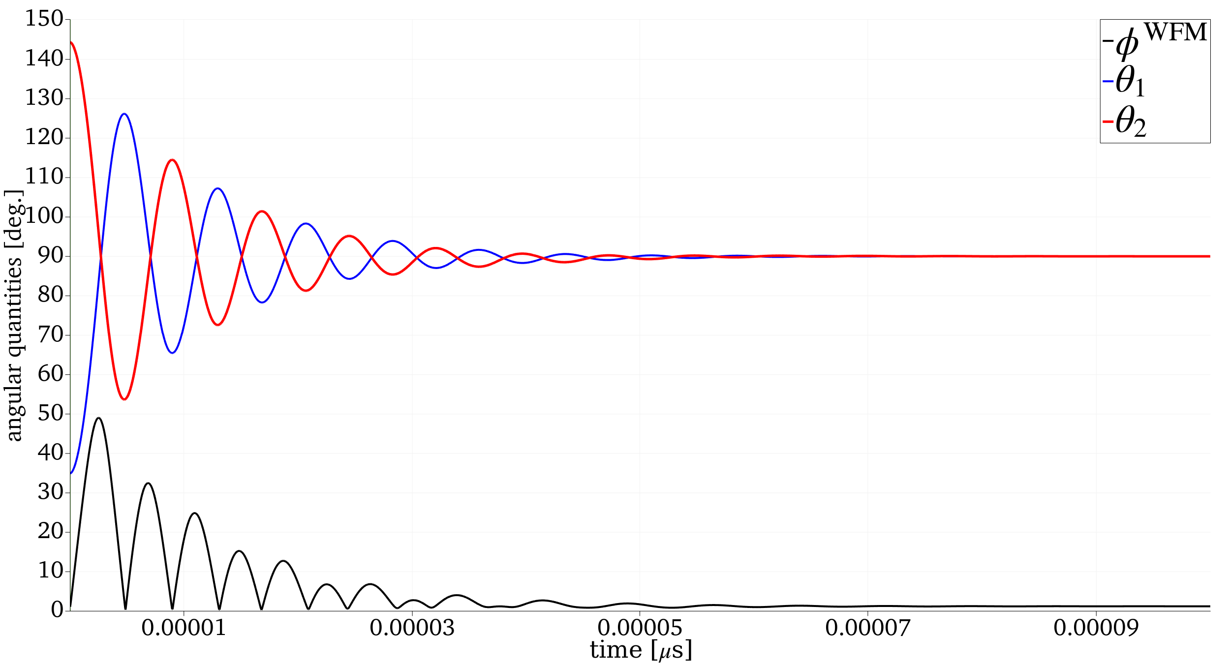
Figure 1: Angular quantities and during ringdown.
By setting the initial condition of in different directions, one can obtain the below table for the eight-fold orientations of .
Importantly, the nonzero value of corresponds to a canted angle of about which agrees well with the literature on BFO.
-------------------------------------------------------------------------------------------------------------------------------------------------------------------------------------------------------
This project SCALES - 897614 was funded for 2021-2023 at the Luxembourg Institute of Science and Technology under principle investigator Jorge Íñiguez-González. The research was carried out within the framework of the Marie Skłodowska-Curie Action (H2020-MSCA-IF-2019) fellowship.

-------------------------------------------------------------------------------------------------------------------------------------------------------------------------------------------------------
References
- Sudipta Biswas, Daniel Schwen, and Jason D. Hales.
Development of a finite element based strain periodicity implementation method.
Finite Elements Anal. Design, 2020.[BibTeX]
- Hemant Dixit, Jun Hee Lee, Jaron T. Krogel, Satoshi Okamoto, and Valentino R. Cooper.
Stabilization of weak ferromagnetism by strong magnetic response to epitaxial strain in multiferroic BiFeO₃.
Sci. Rep., 2015.[BibTeX]
- Natalya Fedorova, Dimitri E. Nikonov, Hai Li, Ian A. Young, and Jorge Íñiguez.
First-principles Landau-like potential for BiFeO₃ and related materials.
Physical Review B, 2022.[BibTeX]