List of tutorials
All tutorials are written assuming that you are reasonably familiar with MOOSE. If you find most of the tutorials difficult to follow, please refer to the official MOOSE website for learning resources.
Tutorial 2: Ferroelectric domain wall
This tutorial gives an example on how to compute the domain wall (DW) profile of (BTO) at room temperature ( K) in FERRET. In this problem (as opposed to Tutorial 1), the polarization is coupled to the elastic strain field via electrostrictive coupling appropriate for BTO. The variable is the component of the elastic displacement vector . The total free energy density is
for the bulk, elastic, gradient, electrostrictive, and electrostatic free energies respectively. The expected DW plane configuration is (100) or equivalent directions so we choose a computational geometry as follows,
[Mesh]
  [gen]
    ############################################
    ##
    ##  Type and dimension of the mesh
    ##
    ############################################

    type = GeneratedMeshGenerator
    dim = 3

    nx = 480
    ny = 1
    nz = 1

    xmin = -60.0
    xmax = 60.0
    ymin = -0.25
    ymax = 0.25
    zmin = -0.25
    zmax = 0.25

    #############################################
    ##
    ##  FE type/order (hexahedral, tetrahedral
    ##
    #############################################

    elem_type = HEX8
  []
  [./cnode]
    input = gen

    ############################################
    ##
    ##   additional boundary sideset (one node)
    ##   to zero one of the elastic displacement vectors
    ##   vectors and eliminates rigid body translations
    ##   from the degrees of freedom
    ##
    ##   NOTE: This must conform with the about
    ##         [Mesh] block settings
    ##
    ############################################

    type = ExtraNodesetGenerator
    coord = '-60.0 -0.25 -0.25'
    new_boundary = 100
  [../]
[]
where and are chosen accordingly such that the mesh spacing nm. In general, the geometry defined in the 'Mesh' block never carries units. The length scale is introduced through Materials, Kernels, or other MOOSE objects. For this problem, the length scale is introduced through the units in the Materials objects that connect to the Kernels. Ferret uses a special base units system (aC, kg, nm, sec) for a number of problems related to ground state prediction. Note that for BTO, . This unit system choice reduces the load quite extensively on the PETSc solvers to iterate the problem. To simulate the DW texture, we choose a profile for with the ICs block inside the Variables block as,
[Variables]

  #################################
  ##
  ##  Variable definitions
  ##    P, u, phi, e^global_ij
  ##  and their initial conditions
  ##
  #################################

  [./global_strain]
    order = SIXTH
    family = SCALAR
  [../]
  [./polar_x]
    order = FIRST
    family = LAGRANGE
    [./InitialCondition]
      type = RandomIC
      min = -0.01e-4
      max = 0.01e-4
    [../]
  [../]
  [./polar_y]
    order = FIRST
    family = LAGRANGE
    [./InitialCondition]
      type = RandomIC
      min = -0.01e-4
      max = 0.01e-4
    [../]
  [../]
  [./polar_z]
    order = FIRST
    family = LAGRANGE
    [./InitialCondition]
      type = FunctionIC
      function = 'stripe1'
    [../]
  [../]

  [./potential_E_int]
    order = FIRST
    family = LAGRANGE
  [../]

  [./u_x]
    order = FIRST
    family = LAGRANGE
  [../]
  [./u_y]
    order = FIRST
    family = LAGRANGE
  [../]
  [./u_z]
    order = FIRST
    family = LAGRANGE
  [../]
[]
where the FunctionIC defines a function called stripe1 with,
Other variables , and are also solved for. This tutorial problem evolves the time-dependent Landau-Ginzburg-Devonshire equation (TDLGD),
to find the ground state with (arbitrary time scale). We also solve (at every time step) the conditions for electrostatic (Poisson equation) and mechanical equilibrium (stress divergence),
with a background dielectric permittivity. The variational derivatives of the total free energy density yield residual and jacobian contributions that are computed within the Kernels block,
[Kernels]

  ###############################################
  ##
  ## Physical Kernel operators
  ## to enforce TDLGD evolution
  ##
  ###############################################

  #Elastic problem
  [./TensorMechanics]
    use_displaced_mesh = false
  [../]

  [./bed_x]
    type = BulkEnergyDerivativeEighth
    variable = polar_x
    component = 0

  [../]
  [./bed_y]
    type = BulkEnergyDerivativeEighth
    variable = polar_y
    component = 1
  [../]
  [./bed_z]
    type = BulkEnergyDerivativeEighth
    variable = polar_z
    component = 2
  [../]

  [./walled_x]
    type = WallEnergyDerivative
    variable = polar_x
    component = 0
  [../]
  [./walled_y]
    type = WallEnergyDerivative
    variable = polar_y
    component = 1
  [../]
  [./walled_z]
    type = WallEnergyDerivative
    variable = polar_z
    component = 2
  [../]

  [./walled2_x]
    type = Wall2EnergyDerivative
    variable = polar_x
    component = 0
  [../]
  [./walled2_y]
    type = Wall2EnergyDerivative
    variable = polar_y
    component = 1
  [../]
  [./walled2_z]
    type = Wall2EnergyDerivative
    variable = polar_z
    component = 2
  [../]

  [./electrostr_ux]
    type = ElectrostrictiveCouplingDispDerivative
    variable = u_x
    component = 0

  [../]
  [./electrostr_uy]
    type = ElectrostrictiveCouplingDispDerivative
    variable = u_y
    component = 1
  [../]
  [./electrostr_uz]
    type = ElectrostrictiveCouplingDispDerivative
    variable = u_z
    component = 2
  [../]

  [./electrostr_polar_coupled_x]
    type = ElectrostrictiveCouplingPolarDerivative
    variable = polar_x
    component = 0
  [../]
  [./electrostr_polar_coupled_y]
    type = ElectrostrictiveCouplingPolarDerivative
    variable = polar_y
    component = 1
  [../]
  [./electrostr_polar_coupled_z]
    type = ElectrostrictiveCouplingPolarDerivative
    variable = polar_z
    component = 2
  [../]

  [./polar_x_electric_E]
    type = PolarElectricEStrong
    variable = potential_E_int
  [../]
  [./FE_E_int]
    type = Electrostatics
    variable = potential_E_int
  [../]

  [./polar_electric_px]
    type = PolarElectricPStrong
    variable = polar_x
    component = 0
  [../]
  [./polar_electric_py]
    type = PolarElectricPStrong
    variable = polar_y
    component = 1
  [../]
  [./polar_electric_pz]
    type = PolarElectricPStrong
    variable = polar_z
    component = 2
  [../]

  [./polar_x_time]
    type = TimeDerivativeScaled
    variable = polar_x
    time_scale = 1.0
  [../]
  [./polar_y_time]
    type = TimeDerivativeScaled
    variable = polar_y
    time_scale = 1.0
  [../]
  [./polar_z_time]
    type = TimeDerivativeScaled
    variable = polar_z
    time_scale = 1.0
  [../]
[]
The weak-form algebra required for setting up these objects are provided in the FERRET syntax list. An interested user may click the hyperlinks here:
TDLGD:
Poisson equation:
Mechanical equilibrium:
TensorMechanics(MOOSEAction) for
for the different objects. Note that the Materials block via
[Materials]

  #################################################
  ##
  ## Bulk free energy and electrostrictive
  ## coefficients gleaned from
  ## Marton and Hlinka
  ##    Phys. Rev. B. 74, 104014, (2006)
  ##
  ## NOTE: there might be some Legendre transforms
  ##        depending on what approach you use
  ##        -i.e. inhomogeneous strain vs
  ##            homogeneous strain [renormalized]
  ##
  ##################################################

  [./Landau_P]
    type = GenericConstantMaterial
    prop_names = 'alpha1 alpha11 alpha12 alpha111 alpha112 alpha123 alpha1111 alpha1112 alpha1122 alpha1123'
    prop_values = '-0.027721 -0.64755 0.323 8.004 4.47 4.91 0.0 0.0 0.0 0.0'
  [../]

  ############################################
  ##
  ## Gradient coefficients from
  ## Marton and Hlinka
  ##    Phys. Rev. B. 74, 104014, (2006)
  ##
  ############################################

  [./Landau_G]
    type = GenericConstantMaterial
    prop_names = 'G110 G11_G110 G12_G110 G44_G110 G44P_G110'
    prop_values = '0.5 0.51 -0.02 0.02 0.0'
  [../]

  [./mat_C]
    type = GenericConstantMaterial
    prop_names = 'C11 C12 C44'
    prop_values = '275.0 179.0 54.3'
  [../]

  ##################################################
  ##
  ## NOTE: Sign convention in Ferret for the
  ##        electrostrictive coeff. is multiplied by
  ##        an overall factor of (-1)
  ##
  ##################################################

  [./mat_Q]
    type = GenericConstantMaterial
    prop_names = 'Q11 Q12 Q44'
    prop_values = '0.11 -0.045 0.029'
  [../]
  [./mat_q]
    type = GenericConstantMaterial
    prop_names = 'q11 q12 q44'
    prop_values = '14.2 -0.74 1.57'
  [../]

  [./eigen_strain]
    type = ComputeEigenstrain
    eigen_base = '0. 0 0 0 0 0 0 0 0'
    eigenstrain_name = eigenstrain
    prefactor = 0.0
  [../]

  [./elasticity_tensor_1]
    type = ComputeElasticityTensor
    fill_method = symmetric9

    ###############################################
    ##
    ## symmetric9 fill_method is (default)
    ##     C11 C12 C13 C22 C23 C33 C44 C55 C66
    ##
    ###############################################

    C_ijkl = '275.0 179.0 179.0 275.0 179.0 275.0 54.3 54.3 54.3'
  [../]
  [./strain_1]
    type = ComputeSmallStrain
    global_strain = global_strain
    eigenstrain_names = eigenstrain
  [../]

  [./stress_1]
    type = ComputeLinearElasticStress
  [../]

  [./global_strain]
    type = ComputeGlobalStrain
    scalar_global_strain = global_strain
    global_strain_uo = global_strain_uo
  [../]

  [./slab_ferroelectric]
    type = ComputeElectrostrictiveTensor
    Q_mnkl = '0.11 -0.045 -0.045 0.11 -0.045 0.11 0.029 0.029 0.029'
    C_ijkl = '275.0 179.0 179.0 275.0 179.0 275.0 54.3 54.3 54.3'
  [../]

  [./permitivitty_1]

    ###############################################
    ##
    ##  so-called background dielectric constant
    ##  (it encapsulates the motion of core electrons
    ##  at high frequency) = e_b*e_0 (here we use
    ##  e_b = 10), see PRB. 74, 104014, (2006)
    ##
    ###############################################

    type = GenericConstantMaterial
    prop_names = 'permittivity'
    prop_values = '0.08854187'
  [../]
[]
We utilize the GlobalStrain system implemented in MOOSE to ensure periodicity of the strain tensor components along the long direction of the box (). This introduces a ScalarKernel,
with the computational volume. We find a set of global displacement vectors disp_x, disp_y, disp_z (see AuxKernels) such that the above condition is satisfied (see Biswas et al. (2020) for an extended description of the method). In the input file, we see a number of objects that allow for this additional system,
[ScalarKernels]

  ######################################
  ##
  ##  Necessary for PBC system
  ##
  ######################################

  [./global_strain]
    type = GlobalStrain
    variable = global_strain
    global_strain_uo = global_strain_uo
    use_displaced_mesh = false
  [../]
[]
and
[UserObjects]

  ###############################################
  ##
  ##  GlobalStrain system to enforce periodicity
  ##  in the anisotropic strain field
  ##
  ###############################################

  [./global_strain_uo]
    type = GlobalATiO3MaterialRVEUserObject
    use_displaced_mesh = false
    execute_on = 'Initial Linear Nonlinear'
  [../]

  ###############################################
  ##
  ##  terminator to end energy evolution when the
  ##  energy difference between subsequent time
  ##  steps is lower than 1e-6
  ##
  ##  NOTE: can fail if the time step is small
  ##
  ###############################################

  [./kill]
    type = Terminator
    expression = 'perc_change <= 1.0e-6'
  [../]
[]
An interested user may click the hyperlink GlobalATiO3MaterialRVEUserObject to see our implementation specific to BTO. The UserObjects also works the the BCs block,
[BCs]
  [./Periodic]
    [./xyz]
      auto_direction = 'x y z'
      variable = 'u_x u_y u_z polar_x polar_y polar_z potential_E_int'
    [../]
  [../]

  # fix center point location
  [./centerfix_x]
    type = DirichletBC
    boundary = 100
    variable = u_x
    value = 0
  [../]
  [./centerfix_y]
    type = DirichletBC
    boundary = 100
    variable = u_y
    value = 0
  [../]
  [./centerfix_z]
    type = DirichletBC
    boundary = 100
    variable = u_z
    value = 0
  [../]
[]
which ensures the appropriate periodicity along the long direction of the box. We find that setting periodicity along the and directions does not influence the system variables and is a redundant boundary condition. This problem also has a number of AuxVariables to store the elastic strain and global displacement fields. Finally, it should be noted that in the UserObjects block, we also include a Terminator object which kills the problem when the relative change of the total energy between adjacent time steps is less than . The wall clock time of this problem is 316.8 secs on 6 processors. After the problem is solved, a typical output can be viewed in ParaView as below.
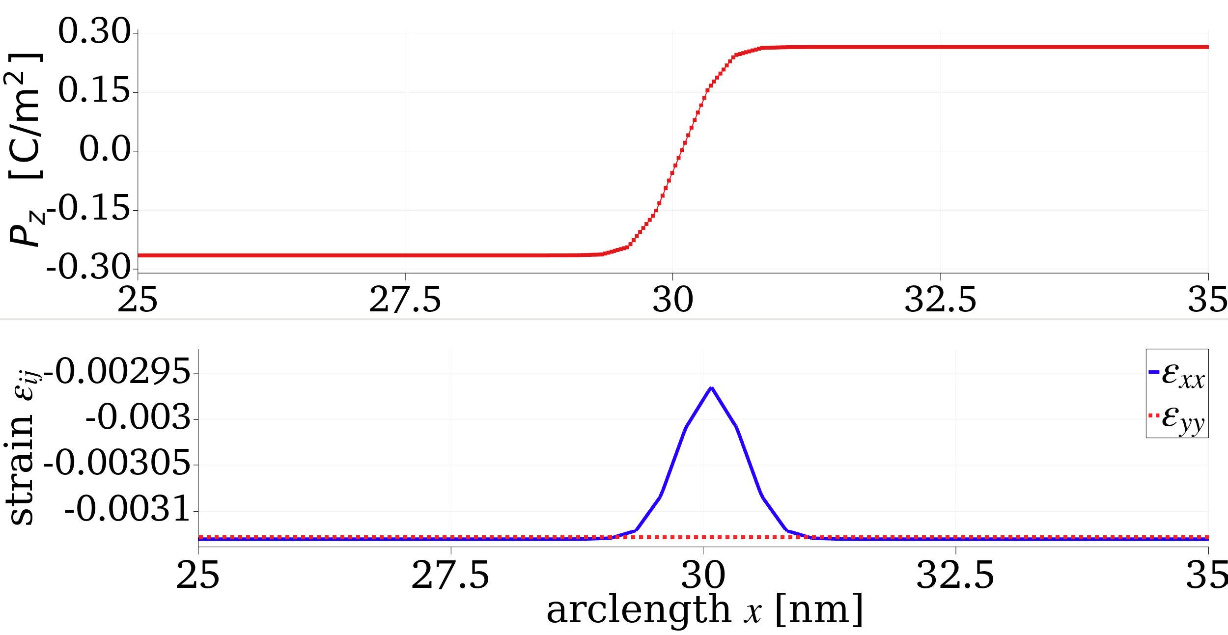
Figure 1: Top: across the DW region. Bottom: Variation of and along the same arclength () in nanometers.
showing the thickness of the DW region along with the variations of the spontaneous strains and . The resulting order parameters in the homogeneous region are , and normal strains and which is in good agreement with the results of Hlinka and Marton (2006). The thickness, which can be calculated by fitting to a profile, agrees well with the calculations from Marton et al. (2010) which highlights a number of a different BTO DWs as a function of temperature.
In principle, this type of calculation can be generalized to any ferroic material (i.e. ferromagnets or multiferroics) to study the DW textures of order parameters in the presence of additional couplings (for example magnetoelasticity or the flexoelectric coupling to gradients in the strain field).
References
- Sudipta Biswas, Daniel Schwen, and Jason D. Hales.
Development of a finite element based strain periodicity implementation method.
Finite Elements Anal. Design, 2020.[BibTeX]
- J. Hlinka and P. Marton.
Phenomenological model of a $90^\circ $ domain wall in BaTiO₃-type ferroelectrics.
Physical Review B, 2006.[BibTeX]
- P. Marton, I. Rychetsky, and J. Hlinka.
Domain walls of ferroelectric BaTiO₃ within the Ginzburg-Landau-Devonshire phenomenological model.
Phys. Rev. B, 2010.[BibTeX]