List of tutorials
All tutorials are written assuming that you are reasonably familiar with MOOSE. If you find most of the tutorials difficult to follow, please refer to the official MOOSE website for learning resources.
Tutorial 4: Ferromagnetic ringdown
This tutorial (and others) covers the basic usage of the micromagnetics implemented in FERRET. This simple problem is for solving the time-dependent LLG equation with exchange stiffness and demagnetizing field phenomena in a permalloy magnet. The total energy density of the system is written as
where and . The coefficient is the exchange stiffness parameter, the saturation magnetization density, and the magnetostatic potential.
We consider a magnetic body with a geometry which we define with the Mesh block.
[Mesh]
  [./mesh]
    type = GeneratedMeshGenerator
    dim = 3
    nx = 50
    ny = 50
    nz = 10
    xmin = -50
    xmax = 50
    ymin = -50
    ymax = 50
    zmin = -10
    zmax = 10
  [../]
  [./vacuum_box]
    type = SubdomainBoundingBoxGenerator
    input = mesh
    bottom_left = '-50 -50 -10'
    top_right = '50 50 10'
    block_id = 2
    block_name = vacuum
  [../]
  [./brick]
    type = SubdomainBoundingBoxGenerator
    input = vacuum_box
    bottom_left = '-10 -10 -1.5'
    top_right = '10 10 1.5'
    block_id = 1
    block_name = brick
  [../]
[../]
In general, the geometry defined in the 'Mesh' block never carries units. The length scale is introduced through Materials, Kernels, or other MOOSE objects. More on this later in this tutorial. Note that the total computational domain is . The remaining area is defined as a vacuum block which acts as a numerical resource in order to solve for the demagnetizing field far from the magnetic body. In principle, we should take the limit which is impossible in a numerical simulation so the volume that is used must be large enough such that the field from the magnetic body naturally goes to zero. We suggest that if the vacuum block approach is used, one should likely test a number of distances to ensure the expected dependence of the demagnetizing field. We use the MOOSE object SubdomainBoundingBoxGenerator to split the mesh into two blocks. In this problem,
[Variables]
  [./mag_x]
    order = FIRST
    family = LAGRANGE
    block = '1'
    [./InitialCondition]
      type = RandomConstrainedVectorFieldIC
      phi = azimuth_phi
      theta = polar_theta
      M0s = 1.0 #amplitude of the RandomConstrainedVectorFieldIC
      component = 0
    [../]
  [../]
  [./mag_y]
    order = FIRST
    family = LAGRANGE
    block = '1'
    [./InitialCondition]
      type = RandomConstrainedVectorFieldIC
      phi = azimuth_phi
      theta = polar_theta
      M0s = 1.0
      component = 1
    [../]
  [../]
  [./mag_z]
    order = FIRST
    family = LAGRANGE
    block = '1'
    [./InitialCondition]
      type = RandomConstrainedVectorFieldIC
      phi = azimuth_phi
      theta = polar_theta
      M0s = 1.0
      component = 2
    [../]
  [../]

  [./potential_H_int]
    order = FIRST
    family = LAGRANGE
    block = '1 2'
  [../]
[]
shows that we are only solving for the variables , and . The initial conditions (ICs) are seeded via spherical coordinates using RandomConstrainedVectorFieldIC to ensure that the ICs satisfy the normalization condition of the LLG equation, .
The micromagnetic problem solves the LLG-LLB equation,
(1)
with . The LLG-LLB equation is partitioned into a few Kernel objects for computation. We separate contributions component-wise and also by specific effective fields (in this case exchange stiffness and demagnetizing fields). These Kernels are listed
[Kernels]
  #---------------------------------------#
  #                                       #
  #          Time dependence              #
  #                                       #
  #---------------------------------------#

  [./mag_x_time]
    type = TimeDerivative
    variable = mag_x
    block = '1'
  [../]
  [./mag_y_time]
    type = TimeDerivative
    variable = mag_y
    block = '1'
  [../]
  [./mag_z_time]
    type = TimeDerivative
    variable = mag_z
    block = '1'
  [../]

  #---------------------------------------#
  #                                       #
  #    Local magnetic exchange            #
  #                                       #
  #---------------------------------------#
  [./dllg_x_exch]
    type = MasterExchangeCartLLG
    variable = mag_x
    component = 0
    mag_x = mag_x
    mag_y = mag_y
    mag_z = mag_z
    block = '1'
  [../]
  [./dllg_y_exch]
    type = MasterExchangeCartLLG
    variable = mag_y
    component = 1
    mag_x = mag_x
    mag_y = mag_y
    mag_z = mag_z
    block = '1'
  [../]
  [./dllg_z_exch]
    type = MasterExchangeCartLLG
    variable = mag_z
    component = 2
    mag_x = mag_x
    mag_y = mag_y
    mag_z = mag_z
    block = '1'
  [../]

  #---------------------------------------#
  #                                       #
  #    demagnetization field              #
  #                                       #
  #---------------------------------------#

  [./d_HM_x]
    type = MasterInteractionCartLLG
    variable = mag_x
    component = 0
    block = '1'
  [../]
  [./d_HM_y]
    type = MasterInteractionCartLLG
    variable = mag_y
    component = 1
    block = '1'
  [../]
  [./d_HM_z]
    type = MasterInteractionCartLLG
    variable = mag_z
    component = 2
    block = '1'
  [../]

  #---------------------------------------#
  #                                       #
  #          LLB constraint terms         #
  #                                       #
  #---------------------------------------#

  [./llb1_x]
    type = MasterLongitudinalLLB
    variable = mag_x
    component = 0
    block = '1'
  [../]
  [./llb1_y]
    type = MasterLongitudinalLLB
    variable = mag_y
    component = 1
    block = '1'
  [../]

  [./llb1_z]
    type = MasterLongitudinalLLB
    variable = mag_z
    component = 2
    block = '1'
  [../]

  #---------------------------------------#
  #                                       #
  #    Magnetostatic Poisson equation     #
  #                                       #
  #---------------------------------------#

  [./int_pot_lap]
    type = Electrostatics
    variable = potential_H_int
    block = '1 2'
  [../]
  [./int_bc_pot_lap]
    type = MagHStrongCart
    variable = potential_H_int
    block = '1'
  [../]

[]
where MasterExchangeCartLLG handles the terms involving the exchange stiffness energy density, MasterInteractionCartLLG involves the interaction with the demagnetizing or applied magnetic fields, MasterLongitudinalLLB is the longitudinal restoring term from the LLB approximation. Finally, we have MagHStrongCart and Electrostatics (the Laplace equation LHS ) for the magnetostatic Poisson equation solved at every time step. The user can click these hyperlinks to see the weak-form algebra necessary to construct the Kernel objects. The Materials block,
[Materials]
  ############################################################################
  ##
  ##       material constants used.
  ##
  ############################################################################

  [./constants]
    type = GenericConstantMaterial
    prop_names = ' alpha           permittivity  Ae        Ms'
    prop_values = '${alphadef}     1.0           1.3e-05   1.2'
    block = '1'
  [../]

  [./a_long]
    type = GenericFunctionMaterial
    prop_names = 'alpha_long'
    prop_values = 'bc_func_1'
    block = '1'
  [../]
  [./constantsv]
    type = GenericConstantMaterial
    prop_names = ' alpha     permittivity Ae      Ms'
    prop_values = '1         1.0        1.3e-05   .0'
    block = '2'
  [../]
  [./a_longv]
    type = GenericFunctionMaterial
    prop_names = 'alpha_long'
    prop_values = 'bc_func_1'
    block = '2'
  [../]

[]
shows the coefficients we will use. Note that is provided to change the time scale of the problem into nanoseconds. A possible visualization output of this tutorial problem using ParaView is provided below
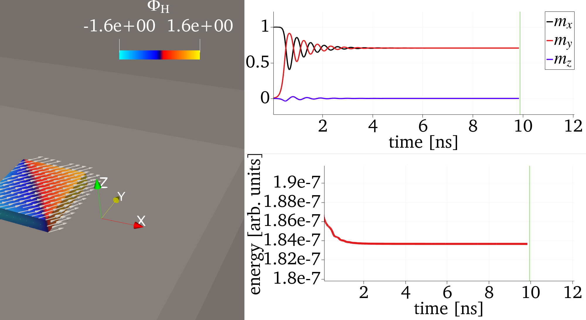
Figure 1: Left: Magnetic (normalized) texture in glyphs and the color map showing the contrast of the demagnetizing potential at the conclusion of the ringdown. The vacuum block is shown as slightly transparent. Top Right: components as a function of time during the ringdown. Bottom Right: Total energy as a function of time.