H2020-MSCA-IF-2019, Example: FE DWs
This page details how to obtain inhomogeneous solutions of BFO for the structural order (i.e. FE DWs). The relevant input file is BFO_dwP1A1_100.i located in the FERRET tutorials subdirectory. The name of the input file is already suggestive, as it identifies that one component of and one component will switch indicating that this is for the 1/1 DW (see Mangeri et al. (2023) on arXiv for more description of this notation). The DW plane is oriented which suggests the plane normal is along . The 1/1 -oriented DW only has large gradients in the components of and . As such, we can simulate this DW profile in quasi 1D with the following Mesh block,
[Mesh]
  [gen]
    type = GeneratedMeshGenerator
    dim = 3
    nx = ${Nx}
    ny = ${Ny}
    nz = ${Nz}
    xmin = 0.0
    xmax = ${xMax}
    ymin = 0.0
    ymax = ${yMax}
    zmin = 0.0
    zmax = ${zMax}
    elem_type = HEX8
  []
  [./cnode]
    input = gen

    ############################################
    ##
    ##   additional boundary sideset (one node)
    ##   to zero one of the elastic displacement vectors
    ##   vectors and eliminates rigid body translations
    ##   from the degrees of freedom
    ##
    ##   NOTE: This must conform with the about
    ##         [Mesh] block settings
    ##
    ############################################

    type = ExtraNodesetGenerator
    coord = '0.0 0.0 0.0'
    new_boundary = 100
  [../]
[]
where xMax, yMax, and zMax define the spatial dimensions of our box. The numbers Nx, Ny, and Nz define the number of finite elements in the calculation. Both of these quantities are listed at the beginning of the input file. We should note that since we are now looking at inhomogeneous structure of and , then the number of finite elements is important. We find that if the spatial discretization is at least nm per element, then the solution is converged to smoothness. The Functions block is important as it allows one to set the initial conditions of and which in the end define the final DW profile,
[Functions]
  [./stripeP1]
    type = ParsedFunction
    value = 0.54*cos(${freq}*(x))
  [../]
  [./stripeP2]
    type = ParsedFunction
    value = -0.54*cos(${freq}*(x))
  [../]
  [./stripeA1]
    type = ParsedFunction
    value = 7.37*cos(${freq}*(x))
  [../]
  [./stripeA2]
    type = ParsedFunction
    value = -7.37*cos(${freq}*(x))
  [../]

  [./constPm]
    type = ParsedFunction
    value = -0.54
  [../]
  [./constPp]
    type = ParsedFunction
    value = 0.54
  [../]
  [./constAm]
    type = ParsedFunction
    value = -7.37
  [../]
  [./constAp]
    type = ParsedFunction
    value = 7.37
  [../]
[]
We pick sin(x) dependence for the initial conditions where the frequency corresponds to where is the length of the box along the long direction. These leads to exactly two DWs in the simulation box. These initial conditions are set explicitly in the Variables block,
!listing tutorial/BFO_dwP1A1_100.i block=Variables link=False language=python
with the FunctionIC MOOSE Object. We evolve the time-dependent Landau-Ginzburg equations,
(1)
where is the total free energy density from that of BFO. As we are not looking for real dynamics of and , we set to unity. We also solve the equation for mechanical equilibrium (Einstein summation convention implied),
which includes the electro- and rotostrictive coupling. The set of these three equations is cast into the weak formulation sufficient for finite element analysis. The set of residual and jacobian contributions are communicated to MOOSE via the Kernels block,
[Kernels]
  [./TensorMechanics]
  [../]

  [./rotostr_ux]
    type = RotostrictiveCouplingDispDerivative
    variable = u_x
    component = 0
  [../]
  [./rotostr_uy]
    type = RotostrictiveCouplingDispDerivative
    variable = u_y
    component = 1
  [../]
  [./rotostr_uz]
    type = RotostrictiveCouplingDispDerivative
    variable = u_z
    component = 2
  [../]

  [./electrostr_ux]
    type = ElectrostrictiveCouplingDispDerivative
    variable = u_x
    component = 0
  [../]
  [./electrostr_uy]
    type = ElectrostrictiveCouplingDispDerivative
    variable = u_y
    component = 1
  [../]
  [./electrostr_uz]
    type = ElectrostrictiveCouplingDispDerivative
    variable = u_z
    component = 2
  [../]

  ### Operators for the polar field: ###
  [./bed_x]
    type = BulkEnergyDerivativeEighth
    variable = polar_x
    component = 0
  [../]
  [./bed_y]
    type = BulkEnergyDerivativeEighth
    variable = polar_y
    component = 1
  [../]
  [./bed_z]
    type = BulkEnergyDerivativeEighth
    variable = polar_z
    component = 2
  [../]

  [./walled_x]
    type = WallEnergyDerivative
    variable = polar_x
    component = 0
  [../]
  [./walled_y]
    type = WallEnergyDerivative
    variable = polar_y
    component = 1
  [../]
  [./walled_z]
    type = WallEnergyDerivative
    variable = polar_z
    component = 2
  [../]
  [./walled2_x]
    type = Wall2EnergyDerivative
    variable = polar_x
    component = 0
  [../]
  [./walled2_y]
    type = Wall2EnergyDerivative
    variable = polar_y
    component = 1
  [../]
  [./walled2_z]
    type = Wall2EnergyDerivative
    variable = polar_z
    component = 2
  [../]

  [./walled_a_x]
    type = AFDWallEnergyDerivative
    variable = antiphase_A_x
    component = 0
  [../]
  [./walled_a_y]
    type = AFDWallEnergyDerivative
    variable = antiphase_A_y
    component = 1
  [../]
  [./walled_a_z]
    type = AFDWallEnergyDerivative
    variable = antiphase_A_z
    component = 2
  [../]

  [./walled2_a_x]
    type = AFDWall2EnergyDerivative
    variable = antiphase_A_x
    component = 0
  [../]
  [./walled2_a_y]
    type = AFDWall2EnergyDerivative
    variable = antiphase_A_y
    component = 1
  [../]
  [./walled2_a_z]
    type = AFDWall2EnergyDerivative
    variable = antiphase_A_z
    component = 2
  [../]

  [./roto_polar_coupled_x]
    type = RotoPolarCoupledEnergyPolarDerivativeAlt
    variable = polar_x
    component = 0
  [../]
  [./roto_polar_coupled_y]
    type = RotoPolarCoupledEnergyPolarDerivativeAlt
    variable = polar_y
    component = 1
  [../]
  [./roto_polar_coupled_z]
    type = RotoPolarCoupledEnergyPolarDerivativeAlt
    variable = polar_z
    component = 2
  [../]
  [./roto_dis_coupled_x]
    type = RotoPolarCoupledEnergyDistortDerivativeAlt
    variable = antiphase_A_x
    component = 0
  [../]
  [./roto_dis_coupled_y]
    type = RotoPolarCoupledEnergyDistortDerivativeAlt
    variable = antiphase_A_y
    component = 1
  [../]
  [./roto_dis_coupled_z]
    type = RotoPolarCoupledEnergyDistortDerivativeAlt
    variable = antiphase_A_z
    component = 2
  [../]

  [./electrostr_polar_coupled_x]
    type = ElectrostrictiveCouplingPolarDerivative
    variable = polar_x
    component = 0
    u_x = disp_x
    u_y = disp_y
    u_z = disp_z
  [../]
  [./electrostr_polar_coupled_y]
    type = ElectrostrictiveCouplingPolarDerivative
    variable = polar_y
    component = 1
    u_x = disp_x
    u_y = disp_y
    u_z = disp_z
  [../]
  [./electrostr_polar_coupled_z]
    type = ElectrostrictiveCouplingPolarDerivative
    variable = polar_z
    component = 2
    u_x = disp_x
    u_y = disp_y
    u_z = disp_z
  [../]

  #Operators for the AFD field

  [./rbed_x]
    type = RotoBulkEnergyDerivativeEighthAlt
    variable = antiphase_A_x
    component = 0
  [../]
  [./rbed_y]
    type = RotoBulkEnergyDerivativeEighthAlt
    variable = antiphase_A_y
    component = 1
  [../]
  [./rbed_z]
    type = RotoBulkEnergyDerivativeEighthAlt
    variable = antiphase_A_z
    component = 2
  [../]

  [./rotostr_dis_coupled_x]
    type = RotostrictiveCouplingDistortDerivative
    variable = antiphase_A_x
    component = 0
    u_x = disp_x
    u_y = disp_y
    u_z = disp_z
  [../]
  [./rotostr_dis_coupled_y]
    type = RotostrictiveCouplingDistortDerivative
    variable = antiphase_A_y
    component = 1
    u_x = disp_x
    u_y = disp_y
    u_z = disp_z
  [../]
  [./rotostr_dis_coupled_z]
    type = RotostrictiveCouplingDistortDerivative
    variable = antiphase_A_z
    component = 2
    u_x = disp_x
    u_y = disp_y
    u_z = disp_z
  [../]

  [./polar_x_electric_E]
    type = PolarElectricEStrong
    variable = potential_E_int
  [../]
  [./FE_E_int]
    type = Electrostatics
    variable = potential_E_int
  [../]
  [./polar_electric_px]
    type = PolarElectricPStrong
    variable = polar_x
    component = 0
  [../]
  [./polar_electric_py]
    type = PolarElectricPStrong
    variable = polar_y
    component = 1
  [../]
  [./polar_electric_pz]
    type = PolarElectricPStrong
    variable = polar_z
    component = 2
  [../]

  [./polar_x_time]
    type = TimeDerivativeScaled
    variable = polar_x
    time_scale = 1.0
    block = '0'
  [../]
  [./polar_y_time]
    type = TimeDerivativeScaled
    variable = polar_y
    time_scale = 1.0
    block = '0'
  [../]
  [./polar_z_time]
    type = TimeDerivativeScaled
    variable = polar_z
    time_scale = 1.0
    block = '0'
  [../]

  [./a_x_time]
    type = TimeDerivativeScaled
    variable = antiphase_A_x
    time_scale = 0.01
    block = '0'
  [../]
  [./a_y_time]
    type = TimeDerivativeScaled
    variable = antiphase_A_y
    time_scale = 0.01
    block = '0'
  [../]
  [./a_z_time]
    type = TimeDerivativeScaled
    variable = antiphase_A_z
    time_scale = 0.01
    block = '0'
  [../]

  [./u_x_time]
    type = TimeDerivativeScaled
    variable = u_x
    time_scale = 1.0
  [../]
  [./u_y_time]
    type = TimeDerivativeScaled
    variable = u_y
    time_scale = 1.0
  [../]
  [./u_z_time]
    type = TimeDerivativeScaled
    variable = u_z
    time_scale = 1.0
  [../]
[]
We direct the reader to the relevant Syntax page for derivations of each of these Kernels and how they relate to the different physics. The total free energy density, , is a fourth-order expansion and contains both contributions from homogeneous phases and also inhomogeneous phases. The latter is introduced as,
and
The relevant materials coefficients (in base S.I. units of nanometers, seconds, attocoulombs, and kilograms) are seeded through the Materials block as,
[Materials]
  [./Landau_P]
    type = GenericConstantMaterial
    prop_names = 'alpha1 alpha11 alpha12 alpha111 alpha112 alpha123 alpha1111 alpha1112 alpha1122 alpha1123'
    prop_values = '-2.81296 1.72351 2.24147 0.0 0.0 0.0 0.0 0.0 0.0 0.0'
  [../]

  [./Landau_A]
    type = GenericConstantMaterial
    prop_names = 'beta1 beta11 beta12 beta111 beta112 beta123 beta1111 beta1112 beta1122 beta1123'
    prop_values = '-0.0137763 0.0000349266 0.0000498846 0.0 0.0 0.0 0.0 0.0 0.0 0.0'
  [../]

  [./P_A_couple]
    type = GenericConstantMaterial
    prop_names = 't1111 t1122 t1212 t42111111 t24111111 t42111122 t24112222 t42112233 t24112233 t42112211 t24111122 t42111212   t42123312 t24121112 t24121233 t6211111111 t2611111111 t6211111122 t2611222222 t4411111111 t4411112222'
    prop_values = '0.012516 0.0180504 -0.036155 0.0 0.0 0.0 0.0 0.0 0.0 0.0 0.0 0.0 0.0 0.0 0.0 0.0 0.0 0.0 0.0 0.0 0.0'
  [../]

  [./Landau_G]
    type = GenericConstantMaterial
    prop_names = 'G110 G11_G110 G12_G110 G44_G110 G44P_G110'
    prop_values = '1.0 ${g11} ${g12} ${g44} 0.0'
  [../]
  [./Landau_H]
    type = GenericConstantMaterial
    prop_names = 'H110 H11_H110 H12_H110 H44_H110 H44P_H110'
    prop_values = '1.0 ${h11} ${h12} ${h44} 0.0'
  [../]

  [./mat_C]
    type = GenericConstantMaterial
    prop_names = 'C11 C12 C44'
    prop_values = '295.179 117.567 74.0701'
  [../]
  [./mat_Q]
    type = GenericConstantMaterial
    prop_names = 'Q11 Q12 Q44'
    prop_values = '-0.0603833 0.0111245 -0.0175686'
  [../]
  [./mat_R]
    type = GenericConstantMaterial
    prop_names = 'R11 R12 R44'
    prop_values = '-0.0000878064 0.0000295306 0.0000627962'
  [../]
  [./mat_q]
    type = GenericConstantMaterial
    prop_names = 'q11 q12 q44'
    prop_values = '-30.4162 -5.01496 -10.4105'
  [../]
  [./mat_r]
    type = GenericConstantMaterial
    prop_names = 'r11 r12 r44'
    prop_values = '-0.0379499 0.00373096 0.0372105'
  [../]
  [./elasticity_tensor_1]
    type = ComputeElasticityTensor
    fill_method = symmetric9
    C_ijkl = '295.179 117.567 117.567 295.179 117.567 295.179 74.0701 74.0701 74.0701'
  [../]

  [./strain]
    type = ComputeSmallStrain
    global_strain = global_strain
  [../]
  [./global_strain]
    type = ComputeGlobalStrain
    scalar_global_strain = global_strain
    global_strain_uo = global_strain_uo
  [../]

  [./stress]
    type = ComputeLinearElasticStress
  [../]

  [./permitivitty_1]

    ###############################################
    ##
    ##  so-called background dielectric constant
    ##  (it encapsulates the motion of core electrons
    ##  at high frequency) = e_b*e_0 (here we use
    ##  e_b = 10), see PRB. 74, 104014, (2006)
    ##
    ###############################################

    type = GenericConstantMaterial
    prop_names = 'permittivity'
    prop_values = '0.08854187'
  [../]
[]
Note that, in principle, our methodology allows for eighth order thermodynamic potentials but the potential relevant for BFO, as parameterized in Fedorova et al. (2022) is of fourth-order. Therefore, there are many zeroes in this Materials block. We also have the Postprocessors block,
[Postprocessors]
  [./dt]
    type = TimestepSize
  [../]
  [./FbP]
    type = BulkEnergyEighth
    execute_on = 'timestep_end'
  [../]
  [./FbA]
    type = RotoBulkEnergyEighth
    execute_on = 'timestep_end'
  [../]
  [./FcPA]
    type = RotoPolarCoupledEnergyEighth
    execute_on = 'timestep_end'
  [../]
  [./FgP]
    type = WallEnergy
    execute_on = 'timestep_end'
  [../]
  [./FgA]
    type = AFDWallEnergy
    execute_on = 'timestep_end'
  [../]
  [./FcPu]
    type = ElectrostrictiveCouplingEnergy
    execute_on = 'timestep_end'
    u_x = disp_x
    u_y = disp_y
    u_z = disp_z
  [../]
  [./FcAu]
    type = RotostrictiveCouplingEnergy
    execute_on = 'timestep_end'
    u_x = disp_x
    u_y = disp_y
    u_z = disp_z
  [../]

  [./Felu]
    type = ElasticEnergy
    execute_on = 'timestep_end'
  [../]
  [./Fele]
    type = ElectrostaticEnergy
    execute_on = 'initial timestep_end'
  [../]
  [./Ftot]
    type = LinearCombinationPostprocessor
    pp_names = 'FbP FbA FgP FgA FcPA FcPu FcAu Felu Fele'
    pp_coefs = ' 1 1 1 1 1 1 1 1 1'
    execute_on = 'timestep_end'

    ##########################################
    #
    # NOTE: Ferret output is in attojoules
    #
    ##########################################
  [../]
  [./perc_change]
    type = EnergyRatePostprocessor
    postprocessor = Ftot
    execute_on = 'timestep_end'
    dt = dt
  [../]

  [./elapsed]
    type = PerfGraphData
    section_name = "Root" # for profiling the problem
    data_type = total
  [../]
[]
which tracks a volume integral over the following free energy density contributions to ,
where is FbP, is FbA, is FcPA, is FgP, is FgA, is FcPu, is FcAu, and is Felu. The Fele quantitity is due to the interaction energy . Also within this block is the summation of all of these energies and a tracker elapsed for wall clock time. The boundary conditions are given by the BCs block,
[BCs]
  [./Periodic]
    [./x]
      auto_direction = 'x'
      variable = 'u_x u_y u_z polar_x polar_y polar_z antiphase_A_x antiphase_A_y antiphase_A_z'
    [../]
    [./xyz]
      auto_direction = 'x y z'
      variable = 'potential_E_int'
    [../]
  [../]
  # fix center point location
  [./centerfix_x]
    type = DirichletBC
    boundary = 100
    variable = u_x
    value = 0
  [../]
  [./centerfix_y]
    type = DirichletBC
    boundary = 100
    variable = u_y
    value = 0
  [../]
  [./centerfix_z]
    type = DirichletBC
    boundary = 100
    variable = u_z
    value = 0
  [../]
[]
This set of BCs along with the GlobalStrain system in MOOSE allows us to have periodicity in the strain tensor components as well as the primary order parameters and . We refer the reader to the tutorial problem Ferroelectric domain wall for more information on the GlobalStrain system. We have the following Executioner options,
[Executioner]
  type = Transient
  solve_type = 'PJFNK'
  scheme = 'bdf2'
  dtmin = 1e-13
  dtmax = 10.0

  [./TimeStepper]
    type = IterationAdaptiveDT
    optimal_iterations = 25 #usually 10
    linear_iteration_ratio = 100
    dt = 0.08
    growth_factor = 1.1
  [../]

  num_steps = 1000
[]
where we implement the backwards- finite difference time integration bdf2 and the preconditioned Jacobi-free Newton-Krylov (PJFNK) method for the solve. A possible visualization of the DW profile in the Exodus output is provided below
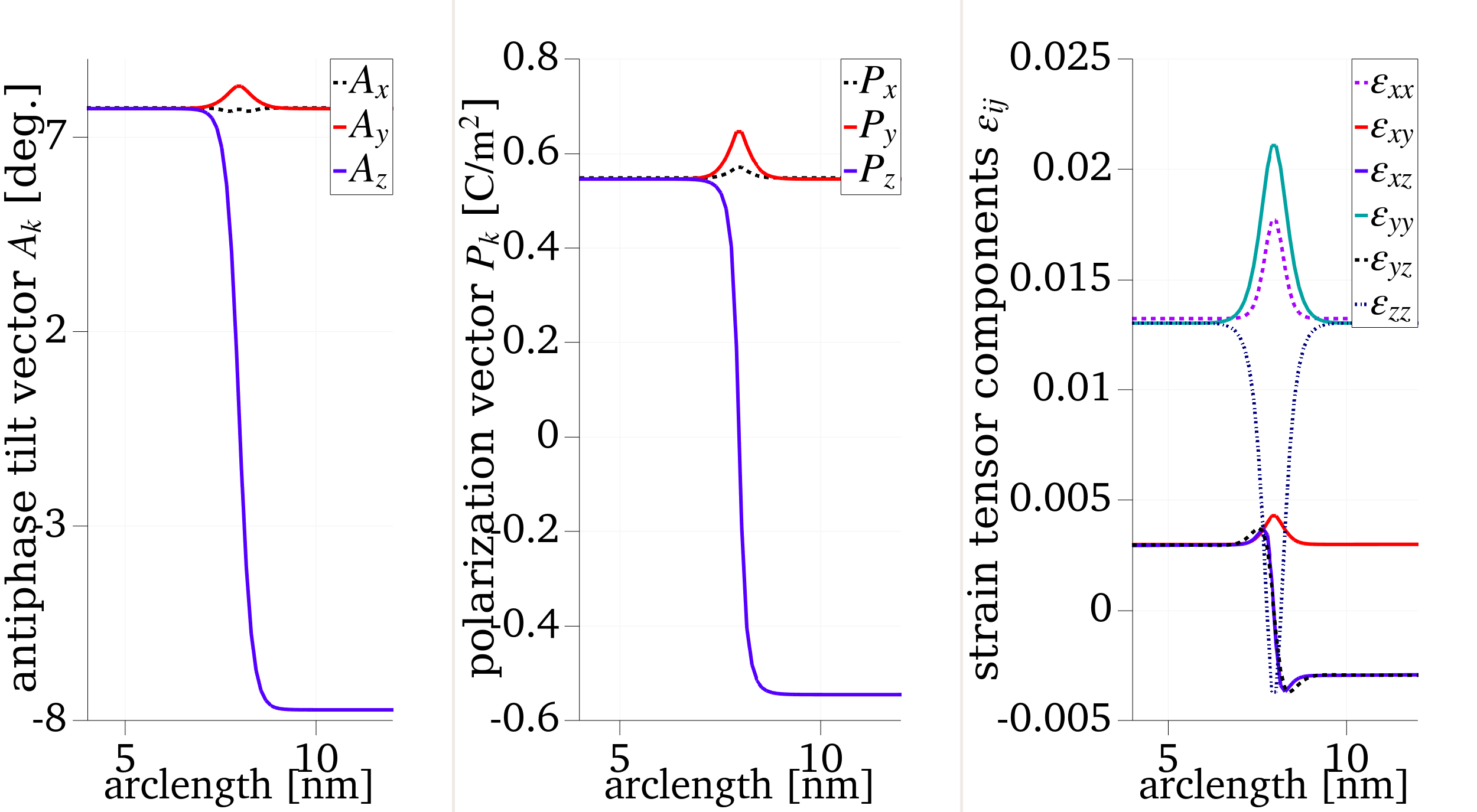
Figure 1: Left: components of , Middle: , and Right: the strain tensor across the DW.
This calculation runs in 68.3 seconds on 6 processors using the WSL distribution of MOOSE. Other DWs can be obtained by switching out the relevant Mesh and Function blocks accordingly.
-------------------------------------------------------------------------------------------------------------------------------------------------------------------------------------------------------
This project SCALES - 897614 was funded for 2021-2023 at the Luxembourg Institute of Science and Technology under principle investigator Jorge Íñiguez-González. The research was carried out within the framework of the Marie Skłodowska-Curie Action (H2020-MSCA-IF-2019) fellowship.

-------------------------------------------------------------------------------------------------------------------------------------------------------------------------------------------------------
References
- Natalya Fedorova, Dimitri E. Nikonov, Hai Li, Ian A. Young, and Jorge Íñiguez.
First-principles Landau-like potential for BiFeO₃ and related materials.
Physical Review B, 2022.[BibTeX]
- J. Mangeri, D. Rodrigues, S. Biswas, M. Graf, O. Heinonen, and J. Iniguez.
A coupled magneto-structural continuum model for multiferroic BiFeO₃.
arXiv:2304.00270, 2023.[BibTeX]