List of tutorials

note:Before you proceed

All tutorials are written assuming that you are reasonably familiar with MOOSE. If you find most of the tutorials difficult to follow, please refer to the official MOOSE website for learning resources.

Tutorial 6: Piezoelectric actuation

This tutorial covers the basic usage of the piezoelectric coupling implemented in FERRET.

In the linear limit, the constitutive governing equation for piezoelectricity is

$\begin{aligned} \frac{\partial}{\partial x_j} \left[C_{ijkl} \left( \varepsilon_{kl} + d_{klm} E_m\right)\right] = 0, \end{aligned}$

where $C_{ijkl}, \varepsilon_{kl},$ and $E_m$ are the components of the elastic stiffness tensor of rank four, elastic strain tensor of rank two, and the electric field vector components. The direct piezoeletric coefficient $d_{klm}$ is of rank three. This is equivalently the equation for mechanical equilibrium with coupling to the electric field, $E_m = - \nabla \Phi_\mathrm{E}$ . Note that the strain tensor is defined in the usual way, $\varepsilon_{kl} = \frac{1}{2} \left( \frac{\partial u_k}{\partial x_l} + \frac{\partial u_l}{\partial x_k} \right).$

Additionally, the Poisson equation also includes contributions from the (converse piezo) strain-charge,

$\begin{aligned} \frac{\partial }{\partial x_r } \epsilon_b \frac{\partial \Phi_\mathrm{E}}{\partial x_r} + \frac{\partial d_{jkl} \sigma_{kl}}{\partial x_j} = 0, \end{aligned}$

with $\sigma_{kl}$ being the components of the elastic stress tensor. With sufficient choice of materials parameters, Equations (1) and (2) can be solved self-consistently under arbitrary mechanical loads or applied electric fields to yield the static configuration of the electrostatic potential and elastic displacements $\mathbf{u}.$

These equations can be cast dynamically, to simulate piezeoelectric actuation in real time. This is done by setting the RHS of the mechanical equilibrium equation to be equal to $\partial u_i / \partial t$

In this problem, we consider a computational geometry

[Mesh]
  type = GeneratedMesh
  dim = 3
  nx = 20
  ny = 10
  nz = 10
  xmin = -10
  xmax = 10
  ymin = -5
  ymax = 5
  zmin = -5
  zmax = 5
  elem_type = HEX8
[]Copy

The finite element mesh discretization schema is chosen to be quadrilateral elements HEX8. In general, the geometry defined in the Mesh block never carries units. The length scale is introduced through Materials, Kernels, or other MOOSE Objects. We seed the materials coefficients $C_{ijkl}$ and $d_{ijk}$ through the following block,

[Materials]
  [./elasticity_tensor_1]
    type = ComputeElasticityTensor
    fill_method = symmetric9
    C_ijkl = '209.7 121.1 105.1 209.7 105.1 210.9 42.47 42.47 44.29'
  [../]
  [./strain_1]
    type = ComputeSmallStrain
  [../]
  [./stress_1]
    type = ComputeLinearElasticStress
  [../]
  [./d333]
    type = ComputePiezostrictiveTensor
    fill_method = general
    e_ijk = '0 0 -0.00415 0 0 0 -0.00415 0 0 0 0 0 0 0 -0.00415 0 -0.00415 0 -0.005 0 0 0 -0.005 0 0 0 0.0124'
  [../]
  [./permitivitty_1]
    type = GenericConstantMaterial
    prop_names = 'permittivity'
    prop_values = '0.0721616'
  [../]
[]Copy

which are given in units of GPa (for $C_{ijkl}$ ). These are typical order of magnitude values of a piezoelectric ceramic. The piezoelectric coefficients carry units of nanometers which sets the length scale of the problem. Also listed is the permittivity of the medium denoted as $\epsilon_b$ and some Materials objects to compute the linear elastic strain and stress. The Kernels suitable for solving the above set of equations are

[Kernels]
  #Elastic problem
  [./TensorMechanics]
    #This is an action block
  [../]
  [./piezocouple_0]
    type = ConversePiezoelectricStrain
    variable = u_x
    component = 0
  [../]
  [./piezocouple_1]
    type = ConversePiezoelectricStrain
    variable = u_y
    component = 1
  [../]
  [./piezocouple_2]
    type = ConversePiezoelectricStrain
    variable = u_z
    component = 2
  [../]
  [./FE_E_int]
    type = Electrostatics
    variable = potential_E_int
  [../]
  [./strain_charge]
    type = PiezoelectricStrainCharge
    variable = potential_E_int
  [../]
[]Copy

which are for the constitutive governing mechanical equations of the piezoelectric (the TensorMechanics Action which sets up $\partial \sigma_{ij} / \partial x_j$ and ConversePiezoelectricStrain which handles the coupling). Also in the Kernels block, we have the Poisson equation, Electrostatics (\nabla^2 \Phi_\mathrm{E}) and PiezoelectricStrainCharge which handles the coupling to the bound charge arising from the strain field. By visiting the hyperlink to the Kernels in the Syntax, we can see how each of these Kernels are constructed as weak form residual contributions.

Finally we have some optional AuxVariables that are computed in

[AuxKernels]
  [./stress_xx]
    type = RankTwoAux
    rank_two_tensor = stress
    variable = stress_xx
    index_i = 0
    index_j = 0
  [../]
  [./stress_yy]
    type = RankTwoAux
    rank_two_tensor = stress
    variable = stress_yy
    index_i = 1
    index_j = 1
  [../]
  [./stress_zz]
    type = RankTwoAux
    rank_two_tensor = stress
    variable = stress_zz
    index_i = 2
    index_j = 2
  [../]
  [./stress_xy]
    type = RankTwoAux
    rank_two_tensor = stress
    variable = stress_xy
    index_i = 0
    index_j = 1
  [../]
  [./stress_yz]
    type = RankTwoAux
    rank_two_tensor = stress
    variable = stress_yz
    index_i = 1
    index_j = 2
  [../]
  [./stress_zx]
    type = RankTwoAux
    rank_two_tensor = stress
    variable = stress_zx
    index_i = 2
    index_j = 0
  [../]
  [./strain_xx]
    type = RankTwoAux
    rank_two_tensor = elastic_strain
    variable = strain_xx
    index_i = 0
    index_j = 0
  [../]
  [./strain_yy]
    type = RankTwoAux
    rank_two_tensor = elastic_strain
    variable = strain_yy
    index_i = 1
    index_j = 1
  [../]
  [./strain_zz]
    type = RankTwoAux
    rank_two_tensor = elastic_strain
    variable = strain_zz
    index_i = 2
    index_j = 2
  [../]
  [./strain_xy]
    type = RankTwoAux
    rank_two_tensor = elastic_strain
    variable = strain_xy
    index_i = 0
    index_j = 1
  [../]
  [./strain_yz]
    type = RankTwoAux
    rank_two_tensor = elastic_strain
    variable = strain_yz
    index_i = 1
    index_j = 2
  [../]
  [./strain_zx]
    type = RankTwoAux
    rank_two_tensor = elastic_strain
    variable = strain_zx
    index_i = 2
    index_j = 0
  [../]
[]Copy

which are stored (i.e. stresses and strains) to be viewed in the output. Some possible outputs of this tutorial problem could look like the figure below using ParaView.

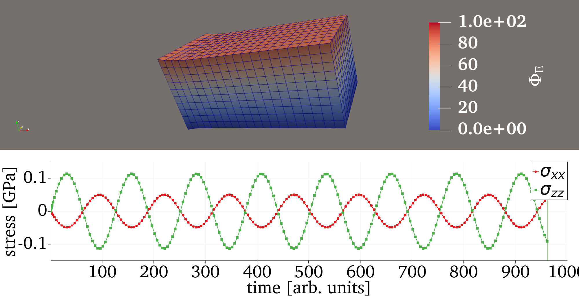
Figure 1: Top: Warped ( $\mathbf{u}$ x100) Filter showing the modulation of the displacement vectors under the applied electric field. Bottom: $\sigma_{xx}$ and $\sigma_{zz}$ components as a function of time during the actuation.

Previous Next