List of tutorials
All tutorials are written assuming that you are reasonably familiar with MOOSE. If you find most of the tutorials difficult to follow, please refer to the official MOOSE website for learning resources.
Tutorial 5: Antiferromagnetic dynamics
This tutorial covers the basic implementation of antiferromagnetic (AFM) dynamics implemented in FERRET. We refer the reader to the first example in Rezende et al. (2019) which considers the unaxial AFM material . The magnetic ion is leading to two sublattices arranged collinearly. The free energy density is,
where and are the effective exchange and anisotropy fields. Only nearest-neighbors along the direction are considered in this example. We evolve the two-sublattice Landau-Lifshitz-Gilbert-Bloch (LLG-LLB) equations,
(1)
where the constant corresponds to the electron gyromagnetic factor equal to GHz, the Gilbert damping, and the longitudinal damping constant from the LLB approximation. The effective fields are defined as with the permeability of vacuum. In this tutorial problem, we look for conservative () time dependent solutions of . This is the linear spin wave excitation limit and this problem is solved analytically in the above reference. The variables are defined as,
[Variables]
  [./mag1_x]
    order = FIRST
    family = LAGRANGE
    [./InitialCondition]
      type = RandomConstrainedVectorFieldIC
      phi = azimuth_phi1
      theta = polar_theta1
      M0s = 1.0 #amplitude of the RandomConstrainedVectorFieldIC
      component = 0
    [../]
  [../]
  [./mag1_y]
    order = FIRST
    family = LAGRANGE
    [./InitialCondition]
      type = RandomConstrainedVectorFieldIC
      phi = azimuth_phi1
      theta = polar_theta1
      M0s = 1.0
      component = 1
    [../]
  [../]
  [./mag1_z]
    order = FIRST
    family = LAGRANGE
    [./InitialCondition]
      type = RandomConstrainedVectorFieldIC
      phi = azimuth_phi1
      theta = polar_theta1
      M0s = 1.0
      component = 2
    [../]
  [../]

  [./mag2_x]
    order = FIRST
    family = LAGRANGE
    [./InitialCondition]
      type = RandomConstrainedVectorFieldIC
      phi = azimuth_phi2
      theta = polar_theta2
      M0s = 1.0
      component = 0
    [../]
  [../]
  [./mag2_y]
    order = FIRST
    family = LAGRANGE
    [./InitialCondition]
      type = RandomConstrainedVectorFieldIC
      phi = azimuth_phi2
      theta = polar_theta2
      M0s = 1.0
      component = 1
    [../]
  [../]
  [./mag2_z]
    order = FIRST
    family = LAGRANGE
    [./InitialCondition]
      type = RandomConstrainedVectorFieldIC
      phi = azimuth_phi2
      theta = polar_theta2
      M0s = 1.0
      component = 2
    [../]
  [../]

[]
where we have used RandomConstrainedVectorFieldIC to set the initial condition such that is on the unit sphere . We choose units of kOe, kOe, and kOe. One can see that the factor of cancels in the above equation so we do not need to set its value other than in the input files. Note that is the strength of an applied field which interacts with the non-equilibrium AFM spins via the Zeeman interaction. If is sufficiently large, a spin flop transition can occur. We choose below this critical value.
This tutorial problem (tutorials/AFMR_MnF2_ex.i) is set up as a macrospin simulation (no spatial gradients). The computational box is simply a finite element grid with m size as shown in the below Mesh block,
[Mesh]
  [gen]
    type = GeneratedMeshGenerator
    dim = 3
    nx = ${Nx}
    ny = ${Ny}
    nz = ${Nz}
    xmin = 0.0
    xmax = ${xMax}
    ymin = 0.0
    ymax = ${yMax}
    zmin = 0.0
    zmax = ${zMax}
    elem_type = HEX8
  []
[]
We seed the coefficients () through the Materials block,
[Materials]
  [./constants_kOe] # Constants used in other material properties
    type = GenericConstantMaterial
    prop_names = ' H0         Ms        g0          He        Ha      '
    prop_values = '8.0e-5    1.0      2.8e9      0.000526     8.2e-6      '
  [../]
  [./constants] # Constants used in other material properties
    type = GenericConstantMaterial
    prop_names = ' alpha     mu0   nx ny nz   long_susc t'
    prop_values = '0.0       1256   0  0  1          1.0     0'
  [../]

  [./a_long]
    type = GenericFunctionMaterial
    prop_names = 'alpha_long'
    prop_values = 'bc_func_1'
  [../]
[]
The value of is set in the ParsedFunction called bc_func_1. In principle, could be time-dependent or depend on spatial coordinates, but for this problem, we just set which is sufficient to constrain . To construct the Kernels relevant for the partial differential equation, we have the following Kernels block,
[Kernels]
  #---------------------------------------#
  #                                       #
  #          Time dependence              #
  #                                       #
  #---------------------------------------#

  [./mag1_x_time]
    type = TimeDerivative
    variable = mag1_x
  [../]
  [./mag1_y_time]
    type = TimeDerivative
    variable = mag1_y
  [../]
  [./mag1_z_time]
    type = TimeDerivative
    variable = mag1_z
  [../]

  [./mag2_x_time]
    type = TimeDerivative
    variable = mag2_x
  [../]
  [./mag2_y_time]
    type = TimeDerivative
    variable = mag2_y
  [../]
  [./mag2_z_time]
    type = TimeDerivative
    variable = mag2_z
  [../]

  #---------------------------------------#
  #                                       #
  #     AFM resonance kernel terms        #
  #                                       #
  #---------------------------------------#

  [./afmr1_x]
    type = UniaxialAFMSublattice
    variable = mag1_x
    mag_sub = 0
    component = 0
  [../]
  [./afmr1_y]
    type = UniaxialAFMSublattice
    variable = mag1_y
    mag_sub = 0
    component = 1
  [../]
  [./afmr1_z]
    type = UniaxialAFMSublattice
    variable = mag1_z
    mag_sub = 0
    component = 2
  [../]

  [./afmr2_x]
    type = UniaxialAFMSublattice
    variable = mag2_x
    mag_sub = 1
    component = 0
  [../]
  [./afmr2_y]
    type = UniaxialAFMSublattice
    variable = mag2_y
    mag_sub = 1
    component = 1
  [../]
  [./afmr2_z]
    type = UniaxialAFMSublattice
    variable = mag2_z
    mag_sub = 1
    component = 2
  [../]

  #---------------------------------------#
  #                                       #
  #          LLB constraint terms         #
  #                                       #
  #---------------------------------------#

  [./llb1_x]
    type = LongitudinalLLB
    variable = mag1_x
    mag_x = mag1_x
    mag_y = mag1_y
    mag_z = mag1_z
    component = 0
  [../]
  [./llb1_y]
    type = LongitudinalLLB
    variable = mag1_y
    mag_x = mag1_x
    mag_y = mag1_y
    mag_z = mag1_z
    component = 1
  [../]

  [./llb1_z]
    type = LongitudinalLLB
    variable = mag1_z
    mag_x = mag1_x
    mag_y = mag1_y
    mag_z = mag1_z
    component = 2
  [../]

  [./llb2_x]
    type = LongitudinalLLB
    variable = mag2_x
    mag_x = mag2_x
    mag_y = mag2_y
    mag_z = mag2_z
    component = 0
  [../]
  [./llb2_y]
    type = LongitudinalLLB
    variable = mag2_y
    mag_x = mag2_x
    mag_y = mag2_y
    mag_z = mag2_z
    component = 1
  [../]

  [./llb2_z]
    type = LongitudinalLLB
    variable = mag2_z
    mag_x = mag2_x
    mag_y = mag2_y
    mag_z = mag2_z
    component = 2
  [../]
[]
There are three FERRET Objects here, which correspond to LongitudinalLLB handling the LLB damping to constrain , TimeDerivative for and UniaxialAFMSublattice which computes the residual and jacobian contributions corresponding to . Note that the LLG-LLB equation for this tutorial problem is hardcoded with Gilbert damping (linear spin wave limit). We refer the reader to the hyperlinks to see the Kernels computations. We also compute and using the VectorDiffOrSum object in the AuxKernels block,
[AuxKernels]
  [./mag1_mag]
    type = VectorMag
    variable = mag1_s
    vector_x = mag1_x
    vector_y = mag1_y
    vector_z = mag1_z
    execute_on = 'initial timestep_end final'
  [../]

  [./mag2_mag]
    type = VectorMag
    variable = mag2_s
    vector_x = mag2_x
    vector_y = mag2_y
    vector_z = mag2_z
    execute_on = 'initial timestep_end final'
  [../]

  [./Neel_Lx]
    type = VectorDiffOrSum
    variable = Neel_L_x
    var1 = mag1_x
    var2 = mag2_x
    diffOrSum = 0
    execute_on = 'initial timestep_end final'
  [../]
  [./Neel_Ly]
    type = VectorDiffOrSum
    variable = Neel_L_y
    var1 = mag1_y
    var2 = mag2_y
    diffOrSum = 0
    execute_on = 'initial timestep_end final'
  [../]
  [./Neel_Lz]
    type = VectorDiffOrSum
    variable = Neel_L_z
    var1 = mag1_z
    var2 = mag2_z
    diffOrSum = 0
    execute_on = 'initial timestep_end final'
  [../]

  [./smallSignalMag_x]
    type = VectorDiffOrSum
    variable = SSMag_x
    var1 = mag1_x
    var2 = mag2_x
    diffOrSum = 1
    execute_on = 'initial timestep_end final'
  [../]
  [./smallSignalMag_y]
    type = VectorDiffOrSum
    variable = SSMag_y
    var1 = mag1_y
    var2 = mag2_y
    diffOrSum = 1
    execute_on = 'initial timestep_end final'
  [../]
  [./smallSignalMag_z]
    type = VectorDiffOrSum
    variable = SSMag_z
    var1 = mag1_z
    var2 = mag2_z
    diffOrSum = 1
    execute_on = 'initial timestep_end final'
  [../]

[]
A possible output of this problem is shown below for the components of as a function of time (in s),
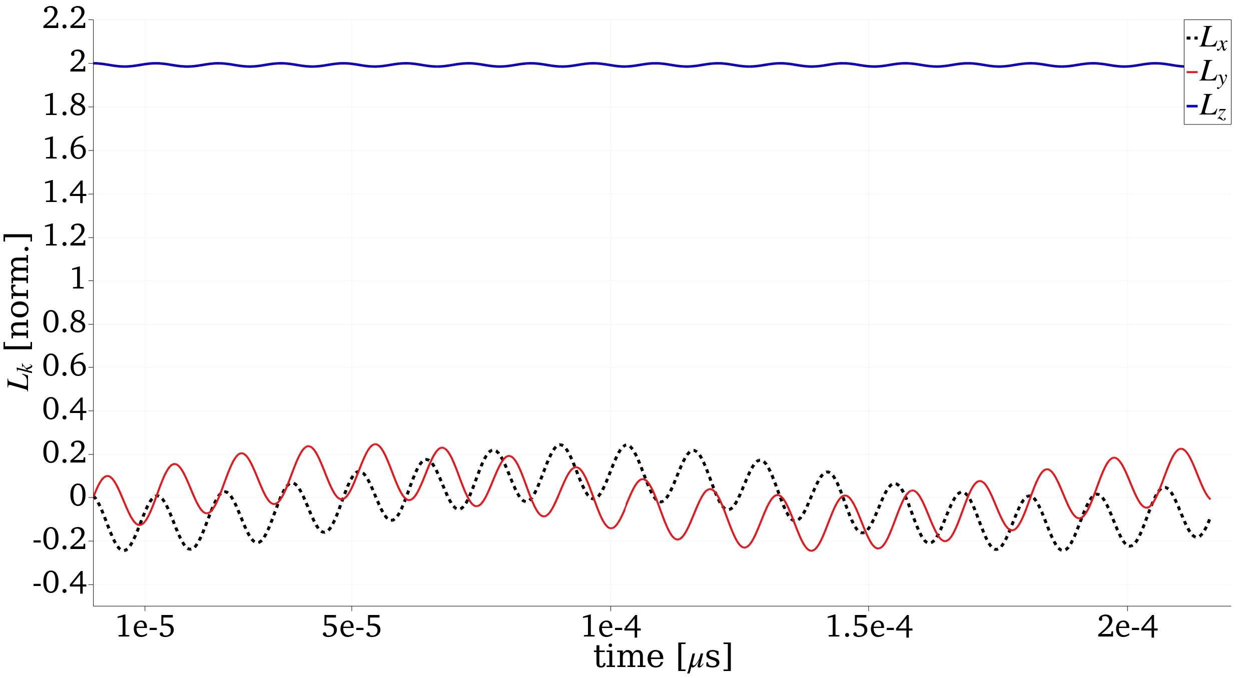
Figure 1: Undamped () evolution of the components of the Neel vector as a function of time of .
It can be seen that the Neel vector components along the direction of the field is relatively constant identifying that the sublattices are precessing about their initial position as expected in the linear limit of the LLG equation. In the article by Rezende et al. (2019), the resonance frequency of the spin sublattice system is calculated analytically as a function of the field strength . We show below good agreement with the results from FERRET for and . We compute two different modes of which correspond to different initial conditions of .
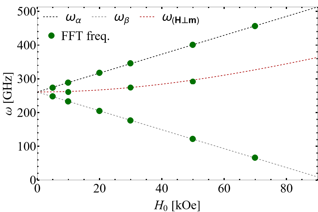
Figure 2: AFM resonance frequency dependence on field strength calculated by FFT from FERRET calculations. The dashed lines correspond to analytical solutions for different modes. See Rezende et al. (2019) for more information.
References
- S. M. Rezende, A. Azevedo, and R. L. Rodríguez-Suárez.
Introduction to antiferromagnetic magnons.
Journal of Applied Physics, 2019.[BibTeX]